In this post we’re going to cover some basic intuition to work on logistic regression for Deep Learning algorithms.
Logistic regression is an algorithm for binary classification, which is basically used when you want to have your model to return 0 or 1. Some examples: is this image a cat? is this email spam? etc.
The basic equation is:
$$
\begin{align}
\hat{y} = w^T x + b \label{basic}
\end{align}
$$
where:
- $\mathbf{\hat{y}}$: is the value that our model predicts
- $\mathbf{w \in \mathbb{R}^n}$: is a vector of $\mathbf{n}$ parameters representing the weights.
- $\mathbf{x \in \mathbb{R}^n}$: is a vector of $\mathbf{n}$ parameters representing the features.
- $\mathbf{b \in \mathbb{R}}$: is a scalar representing the bias or intercept term
$\mathbf{w}$ and $\mathbf{b}$ are the parameters that control the behavior of the model. We can think of $\mathbf{w}$ as the weights that determine how each feature $\mathbf{x_i}$ affects the prediction.
The objective of the machine learning algorithm is to learn the parameters $\mathbf{w}$ and $\mathbf{b}$ so $\mathbf{\hat{y}}$ becomes a good estimate of the chance of being $\mathbf{y}$
Activation function: Sigmoid
The output of the equation ($\ref{basic}$) is a linear function. So, how we transform this linear regression result to a non-linear result? The answer is the sigmoid function that transforms our input to a binary output:
$$
\begin{align}
\hat{y} = \sigma(w^T x + b)
\end{align}
$$
where
$$
\begin{align}
\sigma(z) = \frac{1}{1 + e^{-z}}
\end{align}
$$
The sigmoid function can be represented as:
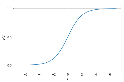
As you can see this activation function allows us to map results to 0 or 1 given:
- For larger positive values of $\mathbf{z}$ we will have a $\mathbf{\sigma(z)}$ near 1
- For larger negative values of $\mathbf{z}$ we will have a $\mathbf{\sigma(z)}$ near 0
Cost Function
First of all, we have the loss function which is used by one training example:
$$
\begin{align}
\mathcal{L}(\hat{y}, y) = - \bigl(y\log\hat{y} + (1 - y) \log(1 - \hat{y})\bigr)
\end{align}
$$
And the cost function measures how you are performing for the entire training set:
$$
\begin{align}
\mathcal{J}(w, b) = \frac1m \sum_{i=1}^m \mathcal{L}(\hat{y}^{(i)}, y^{(i)})
\end{align}
$$
As we want to improve as much as possible the performance, we are going to try to find the w & b values that minimizes this cost function. And that, is basically what gradient descent does for us.
Gradient descent
Gradient descent is one of the most popuar optimization methods for neural networks for its simplicity (although it can have convergence problems due local minimums). Other optimization methods are: Adam or RMSprop.
The basic idea on gradient descent is that on each iteration (determined by the slope or derivative $\partial$), the weights are updated incrementally using a learning rate $\alpha$.
A visual interpretation of gradient descent is the following:

Given our cost function $\mathcal{J}(w, b)$, weights and bias are updated with the following formula:
$$
\begin{align}
w = w - \alpha\,\frac{\partial\,\mathcal{J}(w, b)}{\partial w}
\end{align}
$$
$$
\begin{align}
b = b - \alpha\,\frac{\partial\,\mathcal{J}(w, b)}{\partial b}
\end{align}
$$
where the symbol $\partial$ in $\partial\,\mathcal{J}(w, b)$ basically means the derivative of the cost function.
In the next post, we will see how to apply this theory with an example written with python & TensorFlow.